Two pilot sites give you a DiD number, not a confidence interval
Swap cluster-robust standard errors for backdated and site-permutation placebo tests, then state plainly how little power a small pilot has.
In brief
- When only a few sites are treated, both conventional and cluster-robust standard errors are severely underestimated, so leave them out of the report.
- Use placebo tests instead: move the start date into the past, and assign the pilot role to every pair of control sites.
- A flat pre-trend does not prove parallel trends, and a small number of pilot sites caps the smallest p-value you can reach.
A client lets you deploy a support agent at two of its customer service centers; the other ten carry on as before. Three months later the head of operations asks one question: does the tool actually cut call handling time? Nobody randomized anything at the outset, and two sites are far too few for an A/B test.
This is familiar ground for FDEs. Difference-in-differences (DiD) gives you an impact figure that is easy to explain. The trap lies elsewhere: statistical software will print a neat confidence interval alongside it, and with two sites that interval is almost always narrower than reality.
This guide walks through five steps on a laptop to compute DiD, check it with placebo tests, and write a report that does not promise more than the data can prove. All figures below are hypothetical. The code is a stripped-down version for illustration and uses only pandas and the Python standard library.
What do you need before you start?
You need a long weekly table with the columns site, week, treated (1 for a pilot site) and aht (average handling time, in minutes). The example has 12 sites and 24 weeks, with the pilot starting in week 13 at two sites, S03 and S07. Python 3 and pandas are all you need to install.
Agree with the client in advance on a single metric and the pilot start date. If you choose the metric after seeing the data, every test that follows loses its value.
Step 1: look at the four averages
import pandas as pd

df = pd.read_csv("sites_weekly.csv")   # site, week, treated, aht
START = 13
df["post"] = (df["week"] >= START).astype(int)
print(df.groupby(["treated", "post"])["aht"].mean().unstack())
Check: the printed table must have exactly four cells. Suppose the pilot group falls from 10.0 to 8.6 minutes and the control group from 10.2 to 9.8 minutes. The pilot dropped 1.4 minutes, but the controls also dropped 0.4 minutes, perhaps because of a quiet season or company-wide training. DiD takes the difference between the two drops: −1.4 − (−0.4) = −1.0 minute.
Step 2: wrap the calculation in a function
def did(d, treated_sites, start):
    t = d["site"].isin(treated_sites)
    post = d["week"] >= start
    m = d.groupby([t, post])["aht"].mean()
    return (m[True, True] - m[True, False]) - (m[False, True] - m[False, False])

print(did(df, ["S03", "S07"], START))   # expect ≈ -1.0
The function takes the list of sites and the start date as parameters so that the two placebo steps later on can call it again with fake sites and fake dates.
Step 3: look at the gap week by week, but don’t trust it too much
gap = df.pivot_table(index="week", columns="treated",
                     values="aht", aggfunc="mean")
gap = gap[1] - gap[0]
print(gap.round(2))
Before week 13 the gap between the two groups should hover around a stable level, and only then diverge. This is the eyeball check of the parallel trends assumption: without the pilot, the two groups would have moved in step.
Brantly Callaway, an econometrician who specializes in DiD, points out that parallel trends is an auxiliary assumption that the research design does not guarantee. Pre-intervention data only lets you check it.
Marcus and Sant’Anna go further: pre-intervention coefficients that differ from zero are evidence against the assumption, while failing to reject is not evidence in its favor.
Jonathan Roth adds another layer of warning: pre-trend tests are often underpowered, and continuing the analysis only when the pretest “passes” can itself distort both the estimate and the inference. So use this step to catch obvious problems, not as a free pass.
Why you must not print cluster-robust standard errors
The natural reflex is to run a regression and cluster the errors by site. Alvarez, Ferman and Wüthrich show that when very few units are treated, their observations have high leverage. As a result, both conventional and cluster-robust standard errors are severely underestimated.
With a single pilot site, the authors show that clustering by unit in DiD leads to standard errors that are badly underestimated.
They recommend flatly against reporting cluster-robust SEs in these cases, and suggest the Conley–Taber method or conformal inference. The next two steps are no substitute for those methods.
They are a simplified approach built on an idea that is easy to check: rather than trusting a standard-error formula, you recompute the estimate at times and sites where there was certainly no pilot, then see whether the real figure stands out from the fake ones.
Step 4: move the pilot date into the past
pre = df[df["week"] < START]
for fake_start in [7, 9, 11]:
    print(fake_start, round(did(pre, ["S03", "S07"], fake_start), 2))
You use only the data from before the pilot and pretend it started earlier. There is no real intervention here, so the results should be close to zero.
If a fake date yields −0.8 minutes, your −1.0 minute estimate is measuring something other than the agent. Netflix Games calls this technique backdating and uses it as a robustness check in its synthetic control framework.
Step 5: give the pilot role to each pair of control sites in turn
from itertools import combinations

PILOT = ["S03", "S07"]
real = did(df, PILOT, START)
controls = sorted(set(df["site"]) - set(PILOT))
ctrl = df[df["site"].isin(controls)]          # drop the real pilot sites entirely
placebo = [did(ctrl, list(c), START) for c in combinations(controls, 2)]
p = (1 + sum(abs(e) >= abs(real) for e in placebo)) / (1 + len(placebo))
print(len(placebo), round(p, 3))
The line to watch is ctrl: S03 and S07 are excluded from every fake assignment. If they stayed in, they would sit in the control group of the fake pairs, the agent’s real effect would leak into the comparison, and the placebo estimates would be skewed.
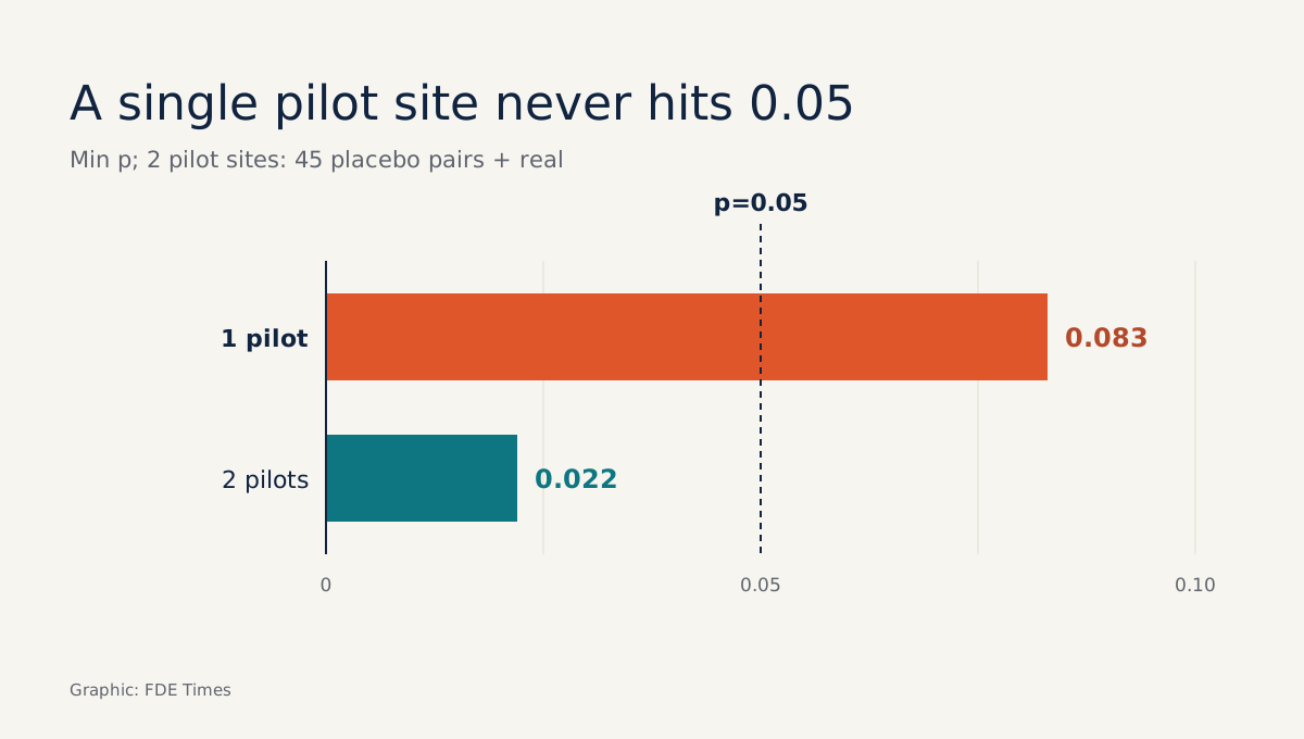
With 10 control sites there are 45 fake pairs. Add the real pair and you have 46 assignments. If −1.0 minute has the largest absolute value, p equals 1/46, about 0.022.
This is a simplified permutation test, not the full procedure from the papers, but its logic is simple enough to explain to a head of operations.
Do one more calculation before promising anything. If the client offers only one pilot site out of 12, you have just 11 fake assignments plus the real one. The smallest possible p is then 1/12, about 0.083, which means you can never reach the 0.05 threshold however well the agent works.
Alvarez and colleagues are explicit on this too: methods that control size correctly can still lack power when the number of treated units is very small.
The most common mistakes
The first is choosing pilot sites by gut feel, usually the ones with the most enthusiastic managers. Those sites may already have been improving, and step 3 will show you this if you look closely.
The second is changing the metric or the start date after seeing the results. The third is pasting a whole regression table with clustered standard errors onto a slide. The number looks professional but is wrong in your favor, which is the kind of error that most easily destroys trust when the client checks it themselves.
How does this skill show up at a client site?
Netflix shows this approach is more than textbook material: it relies heavily on both experiments and quasi-experiments, and uses causal inference on observational data when no A/B test was planned in advance.
The Netflix Games team built a whole framework of synthetic control variants, including synthetic DiD, because each suits a different situation.
On site, the first thing to do is run the step 5 calculation in the pilot design meeting. If there are too few pilot sites to reach the confidence the client needs, negotiate more of them; a longer observation window does not increase the number of ways to assign the pilot role in the permutation test.
Having that conversation before deployment is far easier than explaining a “not statistically significant” result afterwards.
For your career, look for FDE job postings that mention “measure impact” or “prove ROI”. On your CV, instead of “analyzed pilot data”, write that you estimated impact with DiD across N sites, tested it with time and site-permutation placebos, and reported the power limits clearly.
A line like that tells an interviewer you understand both the number and what it cannot prove.
The client will forget the −1.0 minute figure fairly quickly. They will remember longer that you were the one who told them up front how much two sites could prove.
Was this article useful?
Thanks for the feedback!
5 sources
- Inference with few treated units (Alvarez, Ferman, Wüthrich) · 2025-06-25
- Pretest with Caution: Event-Study Estimates after Testing for Parallel Trends (Jonathan Roth, AER: Insights) · 2022-09
- The role of parallel trends in event study settings: An application to environmental economics (Marcus, Sant'Anna) · 2020-09-03
- Difference-in-Differences (Brantly Callaway, Recent Methodological Advances and their Relevance to Empirical Work)
- Round 2: A Survey of Causal Inference Applications at Netflix (mirror of Netflix Technology Blog post) · 2024-06-08