Never quote a Spark cluster size before measuring the customer's data
A number said in the meeting ends up in the budget; a few hours measuring against Spark's defaults shows whether a single machine will do.
In brief
- Spark's default thresholds (128 MB, 200, 10 MB, 2–3 tasks per core) only mean something when set against real measurements from the customer's data.
- For small and medium data, Spark carries a lot of overhead. DuckDB runs on one machine and can spill to disk, making it the comparison worth trying first.
- To conclude that a cluster is needed, you must point to a specific figure that crosses a threshold, such as run time against the batch window.
The second technical meeting with a customer often produces a question like this: “How many nodes should our Spark cluster have?” At that point you have not opened a single one of their data files. Answering on instinct is risky, because a number spoken in a meeting room tends to go straight into the budget.
The safer answer is to ask for one day of real data and a few hours to measure it. This is not dodging the question. Spark’s important settings are all thresholds expressed in bytes, partition counts or cores, so without measurements any number you offer is a guess.
As an FDE, you may have to answer this on an unfamiliar system, with little time, in front of people who do not care what a partition is. You therefore need a measurement routine fast enough to bring numbers to the next meeting.
Spark already has thresholds; your job is to measure the data against them
Spark SQL ships with a few default thresholds to compare your measurements against. When reading Parquet, JSON or ORC, each partition holds at most 128 MB (spark.sql.files.maxPartitionBytes), so input volume determines how many read tasks there are. For joins and aggregations, Spark splits data into 200 shuffle partitions by default (spark.sql.shuffle.partitions).
The third threshold is the broadcast join: a table smaller than 10 MB is sent whole to every worker, so the large table does not have to shuffle. The fourth comes from the tuning guide: Spark recommends 2–3 tasks per CPU core, which means partition counts must be calculated from the cluster’s total core count.
Since Spark 3.2.0, Adaptive Query Execution (AQE) has been enabled by default. AQE uses runtime statistics to re-optimise the plan, coalesces small shuffle partitions towards a default target size of 64 MB, and can split skewed partitions in sort-merge joins.
According to the Spark documentation, AQE means you no longer need to pick a shuffle partition count to fit the dataset. Even so, AQE only fixes the plan at run time. Actual volume, file layout and key skew are still yours to measure.
Measuring a nightly job
Take a hypothetical example. A retail chain runs a nightly job: join the orders table with the stores table, then aggregate revenue by store. You ask for one day of data and run three measurement commands, with nothing to set up.
The first command counts volume and files: aws s3 ls --summarize --recursive s3://customer/orders/date=2026-10-01/. The second uses DuckDB to inspect the Parquet file layout:
SELECT file_name,
       count(DISTINCT row_group_id) AS num_row_groups,
       max(row_group_num_rows)      AS max_rows_per_group
FROM parquet_metadata('orders/*.parquet')
GROUP BY file_name
ORDER BY max_rows_per_group DESC
LIMIT 10;
The third is a PySpark notebook running locally:
from pyspark.sql import functions as F

orders = spark.read.parquet("orders/")
stores = spark.read.parquet("stores/")

print("read partitions:", orders.rdd.getNumPartitions())

total = orders.count()
(orders.groupBy("store_id").count()
   .withColumn("share", F.col("count") / total)
   .orderBy(F.desc("count")).show(10))

orders.cache().count()   # then open the Storage tab in the web UI
(The comment on the last line reads: “then open the Storage tab in the web UI”.)
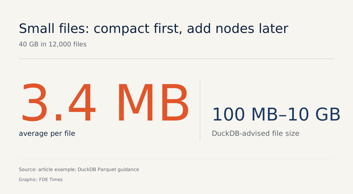
Suppose the results are these: orders weighs 40 GB, split across 12,000 files, averaging about 3.4 MB per file. The stores table is 6 MB. A single store_id, the online sales channel, accounts for 35% of rows. Each result leads to a different decision.
The customer’s files, however, are far smaller than the 100 MB–10 GB range recommended by DuckDB’s Parquet layout guide.
So the first recommendation should be compaction, not more nodes. If the metadata query shows a file with just one giant row group, you also know that file can only be processed by a single thread. A sensible row group holds 100K–1M rows.
At 6 MB, the stores table sits below the 10 MB threshold, so Spark will broadcast it and orders will not have to shuffle for the join. Write this number down: when the customer opens more stores and the table passes 10 MB, the plan will change without anyone telling you.
The key holding 35% is the figure to watch most closely. The Spark documentation states plainly that data skew can severely slow down joins, but AQE’s automatic splitting of skewed partitions applies only to sort-merge joins.
In the web UI, open the aggregation stage and look at the event timeline. One task running far longer than the rest, or a shuffle read many times larger, is the warning sign to raise with the customer in advance.
Last comes memory. The Spark documentation says the best way to estimate it is to cache the dataset and check the Storage page in the web UI. Cache one day of data and you have a real figure to multiply by the period the data must be retained. That number is more reliable than any multiplier rule of thumb.
Does 40 GB need a cluster?
Before considering a cluster, run a comparison. A MotherDuck article observes that for small and medium data, Spark ends up running on its minimum configuration and carrying a lot of overhead.
The article cites AWS Glue as an example: the service requires a minimum of 2 DPUs, so you pay for 32 GB of RAM and 8 vCPUs even when the sample dataset is only about 1 GB.
DuckDB runs on one machine and can still handle data larger than RAM by spilling to disk. So run exactly the nightly job’s join and aggregation on DuckDB, time it, and compare with the customer’s batch window. At the next meeting you bring a measured number rather than an opinion.
For example, if the batch window is 3 hours and DuckDB finishes the 40 GB in 25 minutes, this job does not yet need a cluster.
Only three signals could change that conclusion: single-machine run time approaching the 3-hour window once you factor in the customer’s data growth rate; dimension tables growing large enough that two big tables must be joined; or disk spill taking up most of the run time.
When one of those signals appears, the 2–3 tasks per core recommendation lets you check the configuration with arithmetic. Suppose the planned cluster has 16 cores in total: the matching recommendation is roughly 32–48 partitions.
Only 16 tasks run at any one time, and each core works through two to three tasks in turn, so a core that finishes early picks up the next task instead of sitting idle. Leave shuffle partitions to AQE to coalesce towards the 64 MB target; do not hand-tune the 200.
Common mistakes in the field
The most common mistake is copying the configuration from a previous project, complete with a shuffle.partitions value hand-tuned for an entirely different dataset. The second is measuring on cleaned sample data. A clean sample has no 35% key, so everything runs smoothly during measurement.
The third is looking only at total volume and ignoring file layout. 40 GB in 12,000 small files and 40 GB in 40 files of 1 GB are two different problems. The fourth is forgetting that dimension tables grow. Set an alert when a table approaches 10 MB, because crossing that threshold changes the plan.
Answering the interview question with measurements
One question worth rehearsing before an FDE interview: “A customer has 40 GB of new data every night and asks whether to build a Spark cluster. What do you do?” A weak answer lists tools. A stronger answer sets out a measurement plan.
You can answer in four steps. First, ask for one day of real data and measure volume, file count, row groups, dimension table sizes and key skew. Next, cache a sample to measure real memory.
Then run a single-machine baseline on DuckDB to compare against the batch window. Finally, state clearly which number would make you change your mind. Spend time on this last step: it shows the listener you know when your own conclusion stops holding.
On your CV, write it as a concrete result, for example: “Profiled 40 GB/night of data; recommended compaction and single-machine processing instead of building a cluster.” If a job description mentions infrastructure cost optimisation or system sizing, that is where to tell this story, with the numbers.
Next time a customer asks “how many nodes?”, ask for one day of their data and promise to bring the numbers the following day.
Was this article useful?
Thanks for the feedback!