Anomaly detection on sensor data: build a median and MAD baseline before you train a model

Picture your first week at a customer’s plant. The operations shift lead sends you a CSV of bearing temperatures from twenty pumps and asks: “Can your team do AI anomaly detection?” The temptation is to open a notebook and try an isolation forest or an autoencoder on the spot.

Hold back. What the customer needs in the first month is a rule their engineers can understand, check and adjust themselves when you are not around. A statistical baseline meets all three conditions. It also gives you the yardstick you will later need to prove that a more complex model really does better.

For an FDE this is a very practical skill. Most IoT, infrastructure monitoring and data quality projects start with the question “is this normal?” Whoever can answer it with ten lines of code and a threshold they can explain earns the customer’s trust sooner.

Why the mean and standard deviation mislead you

Grafana Labs, describing how it built anomaly detection on Prometheus, says it started with the formula almost everyone reaches for first: a band of the mean plus or minus a few standard deviations, a variant of the Z-score. That formula works when data is plentiful and clean. Customer sensor data rarely is.

NIST’s statistics handbook warns that the ordinary Z-score can be misleading, particularly with small samples, because the largest Z value that can be reached is limited by the sample size.

The reason is that an anomalous value inflates both the mean and the standard deviation, so it hides itself. Instead, NIST cites the recommendation of Iglewicz and Hoaglin: use the modified Z-score, calculated with the median and the MAD (the median of the absolute deviations from the median).

The formula is M = 0.6745 × (x − median) / MAD. Iglewicz and Hoaglin recommend labelling any point with |M| greater than 3.5 as a “potential outlier”.

Working it by hand with ten readings

Suppose a bearing reports ten temperature readings (°C): 61, 62, 60, 63, 61, 62, 61, 60, 62, 85. Anyone can see that 85 is a problem. The question is whether the formula sees it too.

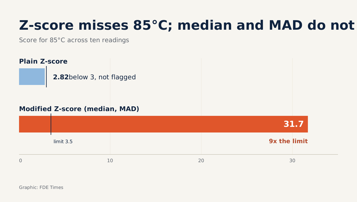
Start with the ordinary Z-score. The sum is 637, so the mean is 63.7. The sample standard deviation is about 7.54, so the Z of the value 85 is 21.3 / 7.54 ≈ 2.82. Against the familiar threshold of 3, the point slips through. Nor could it ever exceed 3: with 10 points, the largest possible Z is only about 2.85, exactly the limit NIST describes.

Now try median and MAD. Sorted, the values are 60, 60, 61, 61, 61, 62, 62, 62, 63, 85, so the median is 61.5. The absolute deviations are six values of 0.5, three of 1.5 and one of 23.5, so the MAD is 0.5.

The value 85 has M = 0.6745 × 23.5 / 0.5 ≈ 31.7, nine times the 3.5 threshold. The value 63 has M ≈ 2.02, so it is not flagged, which is correct.

When the customer asks why you chose the median, one point is enough: a single outlier cannot drag the median anywhere, nor inflate the MAD, so it cannot hide itself the way it does with the mean and standard deviation.

From a hand calculation to a baseline that runs in production

A calculation on ten points is not a system yet. Once it runs continuously you will hit four problems. OneUptime describes the first three in its article on dynamic thresholds; the fourth is the one Grafana had to handle separately when building its Prometheus baseline.

The first problem: an incident leaks into its own baseline. OneUptime suggests offsetting the baseline window by one hour, because the most recent hour is the period most likely to contain an incident in progress.

With a seven-day window, a few dozen minutes of heating will barely move the median. But if you shrink the window to a few hours to react faster, the incident’s data will fill most of the window and can pull the median up with it, so the flag fires late or not at all.

The second problem is the cold start. The same source notes that a new host with one hour of data cannot have a trustworthy seven-day baseline. The same goes for a sensor that has just been installed or replaced, so set a minimum sample count before trusting the baseline.

The third problem follows from that: what do you alert on for a device without enough samples? OneUptime advises keeping a static fallback threshold for resources that have no baseline history yet. In a plant, the natural candidate is the maximum temperature in the manufacturer’s datasheet.

The fourth problem is seasonality. Grafana says it was the last case it had to handle separately, because a simple rolling band was not enough.

It chose a one-hour window after experiments showed this was the right balance for short-term anomaly detection. To smooth the band, it used 26 hours instead of the usual 24, to give users some extra margin.

In a plant, seasonality usually follows the shift pattern. Pumps run under heavy load on the day shift and rest on the night shift, so a simple approach is to calculate a separate baseline for each time slot of the day. Asking the shift lead for the production schedule before you look at the data will save you a week.

import pandas as pd

def flag_anomalies(df, window="7D", offset="1h",
                   min_points=500, static_max=90.0, cutoff=3.5):
    s = df.set_index("ts")["temp_c"].sort_index()
    hist = s.shift(freq=offset)  # baseline does not see the latest hour
    med = hist.rolling(window, min_periods=min_points).median()
    mad = (hist - med).abs().rolling(window, min_periods=min_points).median()
    med = med.reindex(s.index, method="ffill")
    mad = mad.reindex(s.index, method="ffill")
    m = 0.6745 * (s - med) / mad.where(mad > 0)
    has_baseline = med.notna() & mad.gt(0)
    flag = (m.abs() > cutoff) & has_baseline
    fallback = (~has_baseline) & (s > static_max)  # cold start
    return pd.DataFrame({"temp_c": s, "m": m, "flag": flag | fallback})

The rolling MAD here is only an approximation, but it is good enough for a baseline. Note the mad > 0 line: sensors that round to whole degrees often give a MAD of zero during hours when the machine is idle, and dividing by zero would flag the entire morning.

The flag is up. Should you call the customer?

Grafana states plainly that an anomaly on its own is not a strong enough signal that something is broken. A bearing at 85°C could mean a bearing about to fail, but it could also be a scheduled pipeline flush that has just run.

So an anomaly flag is only an input; an alert needs more context: is the machine running, are neighbouring sensors rising too, and has the flag persisted for more than a few cycles?

In meetings with the customer, say “the system saw a point far from its normal level” rather than “the system detected a fault”. The difference sounds small, but it decides whether the customer mutes your alert channel after week two.

The most common mistakes

The most common mistake is using the mean and standard deviation on a handful of points and concluding that “the data has no anomalies”. The second is letting the baseline window reach the present moment, so the incident skews its own baseline. Next comes forgetting the cold start, so every time the customer replaces a sensor there is a burst of false alerts.

The last group of mistakes is human. Some people ignore the shift schedule and flag every machine start-up at 6am. Others push every single flag straight to the customer as a message. Both destroy trust faster than any bad model.

Turning this skill into an edge in interviews

When reading FDE job descriptions, look for phrases such as “industrial data”, “observability”, “time series” or “IoT”. Those are the roles where baseline-building skills get used, so it is worth having a concrete example ready to talk through in interviews.

On your CV, do not write “built an anomaly detection model”. Spell out which threshold you chose and why, how you handled cold starts and seasonality, and how you measured false alerts before and after.

Machine learning models still have their place, but only once the baseline is running and you have numbers to compare against. A model that cannot beat a median and a MAD is not yet fit to go into a customer’s plant.