Demand forecasting: build a baseline and backtest before choosing a model

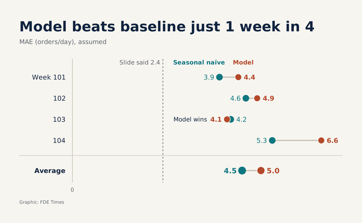
Picture your first week at a logistics company. The head of operations opens a slide: the model forecasting the warehouse’s orders is off by only 2.4 orders a day, and she wants to use it to schedule shifts from next month.

You ask what data that figure was measured on, and the answer is the data the model was trained on. It shows only how well the model remembers the past. It says nothing yet about next week.

Next month, the whole warehouse will work to that number, so you need to pin it down before shifts are locked in. An error here means too many people or too few trucks, not a dashboard metric slightly off, and you should not assume the client’s team has already checked this.

Copying the past is also a model

There are two baselines to build in your first session. With naïve, every forecast equals the last observed value. With seasonal naïve, each forecast equals the most recent value from the same season, which means the same weekday last week if the cycle is one week.

They are not the final answer. The textbook Forecasting: Principles and Practice (FPP3) uses simple methods as benchmarks to ensure a new method is genuinely better, and that is where their value lies: without a baseline, “the model is off by 2.4 orders” tells you nothing.

Now try the arithmetic with hypothetical figures. In week 100, the warehouse receives 100, 95, 98, 102, 130, 180 and 170 orders from Monday to Sunday. In week 101, the actual figures are 104, 99, 96, 106, 128, 186 and 165, and the whole week must be forecast as soon as week 100 closes.

Naïve takes Sunday’s number, so it forecasts 170 orders for all seven days. The total absolute error is 338, an MAE of about 48.3 orders a day. Seasonal naïve copies week 100 straight across, for a total error of only 27 and an MAE of about 3.9.

Error must convert into people and trucks

Clients do not schedule shifts by MAE, so convert it into their units. Suppose one worker can pick 20 orders per shift. With naïve, Monday morning’s forecast is 66 orders too high, which means calling in more than three extra people; with seasonal naïve, the average error of 3.9 orders is less than one person.

Trucks work the same way. Suppose each truck carries 30 orders: naïve’s 66 surplus orders mean more than two trucks booked for nothing, while seasonal naïve’s worst day is off by just 6 orders, a fifth of a truck.

To make that conversion, you have to ask the operations people at the outset: which decision does this forecast serve, how far ahead is it locked in, and at what level? If shifts are locked in 7 days ahead, the horizon is 7 days, and every measurement must use that horizon.

FPP3 also notes that one-step errors may not be relevant when multi-step forecasts are needed, and that the evaluation procedure can be adjusted to measure error at step h. An error measured one day ahead is no help to someone scheduling shifts a week ahead.

A backtest has only one hard rule

Rob Hyndman describes this evaluation through the image of a forecast origin rolling forward in time. Its rule is compact: the training set contains only observations that occurred before the observation used for testing. The errors are then averaged across the test sets.

Take 104 weeks of history and four 7-day windows. The calculation above is the first window: train through the end of week 100 and score on week 101. The last window trains through week 103 and scores on week 104, so the training set grows with each pass, just as scikit-learn’s TimeSeriesSplit works.

The code runs to only about 20 lines. Write it by hand once to see exactly where the data is cut, and make the forecasting function a parameter so that every method is scored on the same windows:

import numpy as np
import pandas as pd

def naive(train, h):
    return [train.iloc[-1]] * h

def seasonal_naive(train, h, season=7):
    # assumes h <= season
    return train.iloc[-season:].values[:h]

def backtest(y, forecast_fn, h=7, n_windows=4):
    # y: daily pd.Series, sorted by time, with no missing days
    rows = []
    for w in range(n_windows, 0, -1):
        cutoff = len(y) - w * h
        train = y.iloc[:cutoff]              # only data before the origin
        test = y.iloc[cutoff:cutoff + h]
        forecast = np.asarray(forecast_fn(train, h))
        mae = abs(test.values - forecast).mean()
        rows.append({"start": y.index[cutoff], "mae": mae})
    return pd.DataFrame(rows)

Each call to backtest returns its own DataFrame, so merge them on the start date to get two columns to compare:

comparison = backtest(y, naive).merge(
    backtest(y, seasonal_naive),
    on="start",
    suffixes=("_naive", "_seasonal"),
)

To test the client’s model, wrap it in a function that takes train and h, retrains on train in each window and returns h forecast values. Then merge its results in the same way.

When the client has many series, do not keep extending this loop yourself. Nixtla’s StatsForecast documentation describes cross-validation as a window sliding over the history and forecasting the period immediately after it, with step_size as the gap between windows, meaning how often the forecast is run. Set it to match the client’s shift-locking rhythm.

Amazon Forecast measures in the same way: the service’s documentation uses backtests to evaluate a predictor’s accuracy. The four windows in the table below are cut down to keep things easy to follow; with 104 weeks of history, you have enough data to run more before reaching a conclusion.

7-day window	Seasonal naïve MAE	Client model MAE
1 (week 101)	3.9	4.4
2 (week 102)	4.6	4.9
3 (week 103)	4.2	4.1
4 (week 104)	5.3	6.6
Average	4.5	5.0

These are still hypothetical numbers, but read them as you would in front of the client. The model that boasted 2.4 orders now misses by an average of 5.0 when it has to make real forecasts, loses to the baseline’s 4.5 and wins only one window in four. Window 4 is the first place to look, because that is where the gap is widest.

These four weeks may be too calm, so do not decide yet. Run more windows covering the peak weeks in the 104 weeks of history, and only then make a recommendation.

If the result stays the same, what you should tell the head of operations is very short: “The model does not yet beat copying last week. Next week we can schedule shifts with the baseline, and the model goes in when it beats that baseline on this same measure.” You are not wrecking anyone’s project. You are giving the client an option that works right away and a measurable target.

If the result goes the other way and the model wins most windows, convert the difference into people and trucks before discussing deployment. The client then knows what they gain over the cheapest approach.

MASE below 1 is not yet a win

In this example, MASE divides the model’s error by the average error of one-step naïve on the training data. According to FPP3, a result below 1 means better than the average one-step naïve forecast, and above 1 means worse.

Hyndman and Koehler proposed MASE as a standard measure for comparing accuracy across multiple series. The metric is genuinely convenient, but a figure below 1 can easily make readers celebrate too early.

Take window 1, training through the end of week 100 and scoring on week 101. For simplicity, assume the day-to-day difference across all the training data exactly matches that of week 100: the six differences add up to 100, an average of about 16.7.

The model misses by 4.4 orders, giving a MASE of about 0.26, which sounds very impressive. Seasonal naïve misses by 3.9 orders and scores about 0.23, so it still beats the model.

The 0.26 does not prove the model is good. This series has a clear weekly cycle, and the weekend jumps inflate the one-step denominator, so getting below 1 is fairly easy.

So always report MASE next to the seasonal naïve figure, and never let it stand alone. When reading numbers from your own tools, also check which denominator they use before comparing them with this article.

The mistakes that make a backtest pretty but useless

The first mistake is using random K-fold out of habit. The scikit-learn documentation explains why this is wrong for time-ordered data: the model would learn from the future and then be scored on the past.

Even with the data cut correctly, leakage can still come through features. Rolling averages or normalisation computed on the full series carry the future into the past; so does a promotion calendar finalised late, if it would not exist at real forecast time. Ask of each feature: on the day shifts are locked in, does this number exist yet?

Another trap is choosing windows that are too calm. A few ordinary weeks say nothing about how the model will behave in a peak week, so a backtest needs to cover peak seasons and periods when operations changed.

Reading the results has traps of its own. A single window may be just one lucky week, and an average can hide the worst window, so look at the full window-by-window table before concluding.

The remaining trap lies in the client’s own data. Zero sales on a stockout day does not mean zero demand, and you will teach the model the wrong thing if those days are not flagged. Check against inventory history before trusting the sales series.

Work in the right order, then put real numbers on your CV

In your first week, settle the horizon with the operations people first, then get the baseline running before anyone starts discussing model architecture.

When writing your CV, do not just list algorithm names. Describe the work, such as “multi-window backtest at a 7-day horizon, reducing MAE against seasonal naïve”, with your own real numbers.

When reading a job description that mentions forecasting or supply chain, ask which baseline they compare their model with; in interviews, bring up the baseline before you are asked.

The next time someone shows off a handsome error figure, do not ask which model they used. Ask: how does it compare with last week?